1. Introduction
This is the documentation for COVE, the COastal Vector Evolution model - a vector-based one-line coastal evolution model. The model was presented and used in a paper on the evolution of crenulate bays published in the Journal of Geophysical Research Earth Surface (Hurst et al., 2015). The model is intended for research purposes, exploring coastal behaviour and sensitiviy.

Development of COVE was lead by Martin D. Hurst at the British Geological Survey as part of a National Capability project to explore Environmental Sensitivity and Change within the Land, Soil and Coast Research Program directed by Michael A. Ellis. Development of COVE was also supported by the NERC and Environment Agency funded iCOASST Project.
The model is intended for research purposes. It is released under a GNU General Public Licence. If you are interested in working with COVE, we would encourage you to get in touch and work with us. In this introduction, we will give a brief overview of the science behind the model.
Reference documentation for the code has been generated using Doxygen and the resulting reference material can be accessed at COVE Doxygen Documentation.
SUMMARY
-
COVE is a ‘one-line’ type shoreline evolution model.
-
Application at spatial scales of kms to tens of kms, over decadal to millennial timescales.
-
Coastal change is driven by gradients in wave-generated alongshore sediment transport.
-
Alongshore sediment transport driven by the height and angle of breaking waves.
-
Produces emergent landforms (such as capes and spits) and processes (wave shadowing)
-
Retreat of cliffs governed by beach interaction (protection vs tools).
1.1. Overview
The COVE model is a special case of a ‘one-line’ model designed to handle complex coastline geometries, with high planform curvature shorelines (Hurst et al., 2015). The shoreline is represented by a single line (or contour) that advances or retreats depending on the net alongshore sediment flux. COVE is now actually a two-line model because a second line representing coastal cliffs interacts with the shoreline, eroding to provide beach sediment. One-line models make a number of simplifying assumptions to conceptualise the coastline allowing the ‘one-line’ representation of the coastline:
ASSUMPTIONS
-
Short-term cross-shore variations due to storms or rip currents are considered temporary perturbations to the long-term trajectory of coastal change (i.e. the shoreface recovers rapidly from storm-driven cross-shore transport).
-
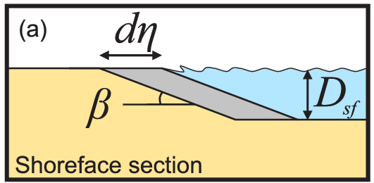
The beach profile is thus assumed to maintain a constant time-averaged form (Fig. 1), implying that depth contours are shore-parallel and therefore allows the coast to be represented by a single contour line.
-
Alongshore sediment transport occurs primarily in the surf zone, and cross-shore sediment transport acts to maintain the equilibrium shoreface as it advances /retreats.
-
Alongshore sediment flux occurs due to wave action in the surf zone, parameterized by the height and angle of incidence of breaking waves. Gradients in alongshore transport dictate whether the shoreline advances or retreats.
1.2. Governing equation
Previous one-line models have cast the conservation of sediment in a gridded cartesian framework, relative to the general orientation of the coastline (the \(x\)-coordinate). The result is that coastal cells are rectangular and either prograde or regress perpendicular to the general orientation of the coastline (the \(y\)-coordinate):
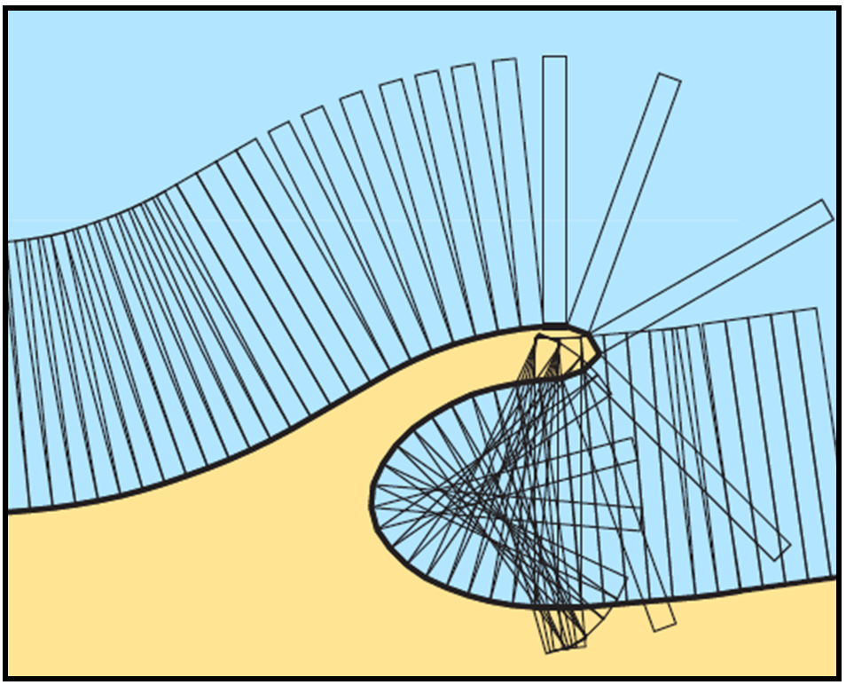
image::rectangular_cells.png[title="Schematic planform diagram of a coastline with rectilinear cells orientated perpendicular to the general trend of the shoreline, as assumed in one-line models. The shoreline either advances or retreats in the \(y\) direction",width="300",align="center"]
Given the assumption that the evolution of the coastline is driven by gradients in alongshore sediment transport, the conservation equation for this setup (e.g. Ashton and Murray, 2006) states that the change of position of the coast \(y\) is equal to the divergence in alongshore sediment flux \(Q_{ls}\) divided by the shoreface depth \(D_{sf}\):
\(\frac{dy}{dt} = \frac{1}{D_{sf}}\left(\frac{dQ_{ls}}{dx}\right)\)
However, when the shoreline has high planform curvature, this equation becomes difficult to apply as the principle of conservation of mass is violated. Ashton and Murray (2006) dealt with this problem through the use of a cellular model. Alternatively, it has been proposed to use a local coordinate system (LeBlond, 1972; Kaergaard and Fredsoe, 2013).
1.2.1. Using a local coordinate system
The conservation equation for beach sediment expressed in terms of local coordinates states that the change in position of the shoreline \(d\eta\), perpendicular to the local shoreline orientation \(s\) through time \(t\) is a function of the divergence of alongshore sediment flux \(Q_{ls}\):
\(\frac{d\eta}{dt} = f\left(\frac{dQ_{ls}}{ds}\right)\)
1.3. Cell building routine
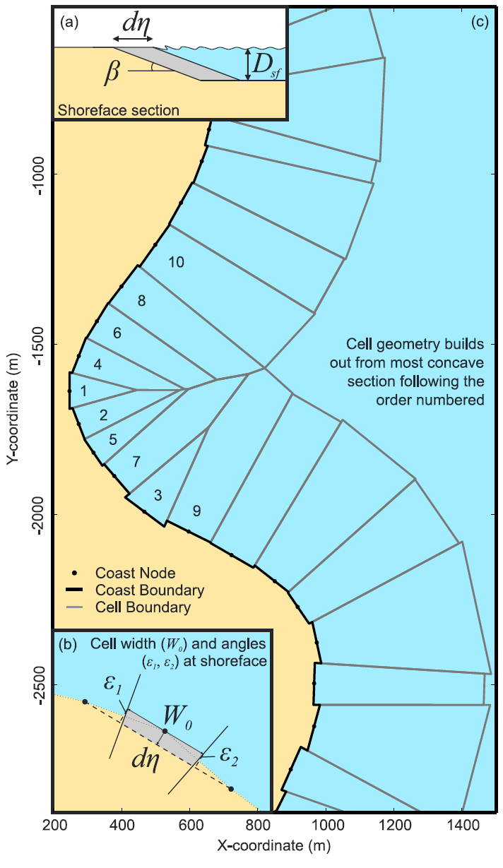
1.3.1. Irregular shoreline cells
The nature of the conservation of mass function is dependent on the geometry of shoreline cells. If we were to use rectilinear cells we would violate mass conservation because the cells would either diverge or converge offshore, depending on the planform curvature of the shoreline (i.e. convex offshore vs concave offshore respectively).
In COVE, coastline cells are not rectilinear, but rather triangular, trapezoidal or polygonal. The change of shoreline position for such cells is calculated by inverting quadratic and cubic equations for the volume of sediment in these cells (see Hurst et al., 2015).
1.3.2. Cell geometry
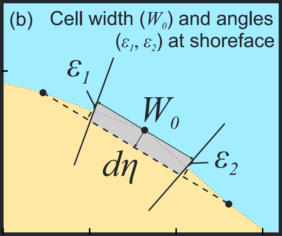
Each coastline node has an orientation calculated as the azimuth angle of a vector connecting the two adjacent nodes. Cell edges seperating adjacent cells have an orientation that is perpendicular to imaginary lines between the node of interest and each adjacent node, and they bisect these lines. The cell is thus defined by the cell width at the shoreline \(W_0\), and two angles describing the difference between the cell orientation and the cell boundary orientations \(\eta_1\) and \(\eta_2\) for the upcoast and downcoast boundaries respectively.
1.3.3. Mesh building algorithm
The model builds coastal cells by projecting offshore the cell edges defined above. The procedure is as follows: . A priority queue is built so that cells with the largest value of latexmath:[\eta_1+eta_2] are prioritised. . Starting with the most acute, cell boundaries are projected offshore until… .. They intersect, in which case the cell is closed and a new boundary for adjacent cells will be created from the intersection point, and adjacent cells will be added to the priority queue again; or .. The bottom of the shoreface \(D_{sf}\) is reached and the cell is closed by a straight line across the shoreface defining the bottom of the shoreface. . The procedure continues until all cells have been meshed.
1.4. Alongshore Flux
Bulk alongshore sediment flux is driven by waves breaking on the shoreface. Typically in alongshore transport laws, flux depends on the height \(H_b\) and angle \(\alpha_b\) of breaking waves. For example, in the simplest case of fine/medium sand, COVE uses the CERC equation:
\(Q_{ls} = K_{ls} H_b^{5\over2} \sin 2\alpha_b\)
where \(K_{ls}\) is a transport coefficient. The transport coefficient \(K_{ls}\) may be modified to account for the size of beach material (\(D_{50}\)). Calibration of this coefficient can be made from estimates of bulk alongshore transport or by calibration against a historical record of coastal change (e.g. Barkwith et al. 2014a).
1.5. Cliff Erosion
Cliffs are represented in the model as a separate line. The cliffline and coastline interact to determine how wide the beach is locally. Eroded cliff material is provided to the adjacent beach and causes the shoreface to advance. Cliff erosion is controlled by beach width since a wider beach provide energy dissipation and protection from approaching waves. Figure 2 shows a schematic graph of this relationship, as well as a conceptual diagram of the representation and relationship of the cliff and the beach.
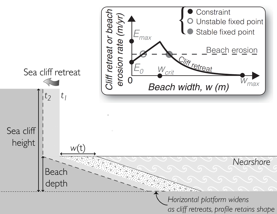
The result is that we can run simlutaions at decadal timescales to explore the interactions between coastal erosion and alongshore sediment dynamics.
1.6. Model requirements
1.6.1. Data
-
The model requires offshore wave data. Offshore in this case is defined as waves that are unaffected by refraction, shoaling and shadowing at the shoreface. This can be obtained either from a wave buoy or preferably from distributed coastal area modelling predictions of wave conditions (e.g. FVCOM or SWAN).
-
The transport coefficient \(K_{ls}\) may be modified to account for the size of beach material (\(D_{50}\)). Calibration of this coefficient can be made from estimates of bulk alongshore transport or by calibration against a historical record of coastal change.
-
Historical shoreline positions and legacy wave data allow training of the model to reproduce past geomorphic changes.
1.6.2. Boundary Conditions
-
Offshore waves (see above).
-
Coupling to sediment sources and sinks (e.g. river mouth, estuary).
-
Human interaction with the coast (e.g. Barkwith et al. 2014b):
-
Nourishment can be provided to build out the shoreface
-
Hard defences represented as immovable, cliffed shoreline
-
Groin fields simulated by prescribing a minimum beach width
-
2. Software Requirements
COVE is written in C++, partly for efficiency but also to allow us to take advantage of running ensembles of simulations on UNIX high performance computing (HPC) clusters. The code has been written and tested extensively in a Linux/UNIX environment, and has also been compiled and run on Windows using Code::Blocks, but has not been tested on Mac. So for now, you`re going to need to be/get familiar with working at a command line interface.
There are a number of software requirements to run the model and visualise the results.
-
C++ compiler (e.g. GCC: the GNU Compiler Collection)
-
Text editor (e.g. gedit, Notepad++)
-
Python + Scipy, Numpy and Matplotlib packages
2.1. Linux/UNIX
If you do not already work in Linux or UNIX, then the easiest way to get started would be to use some virtualisation software such as VirtualBox or VMWare Workstation Player. VirtualBox is preferable since it is open source and free to use, but there are some minor advantages to using VMWare Player if you become a heavy user. We hope soon to provide a Vagrant file to make this process a bit more straight forward. For now, I recommend installing VirtualBox, creating a new virtual machine, and installing Ubuntu using a downloaded iso file.
2.1.1. Git
Git is version control software. The model is stored in a repository on github. This allows us to track all of our updates and developments and avoid duplication. You can install git from the command line:
$ sudo apt-get install git
Getting to grips with git can be a steep learning curve at first. The github glossary is useful for getting up to speed with the terminology, and I found a good cheat sheet for git commands.
2.1.2. C++ Compiler
If you are using a Linux machine (e.g. the recommended Ubuntu VM) then you should have the GNU Compiler Collection installed. Depending on your experience and whether your developing the model, the GNU debugger can also be helpful (should already be installed with GCC), not to mention Valgrind (you probably know what you`re doing better than I do if you`re using Valgrind!). We will also need the make utility (this should also be ready installed). No additional C++ libraries are required at this stage.
2.1.3. Text editor
A text editor is required for viewing and editing both the main code and driver files (shorter bits of code that interact with and control the main model objects). Ubuntu ships with gedit, which I find works well once you install and activate some useful plugins.
$ sudo apt-get install gedit-plugins gedit-developer-plugins
Some of these can really increase productivity while writing code.
2.1.4. Python
Python is a programming language that is great for analysing and visualising data, and is used here to visualise the output of COVE and running further analyses on model results. Again Python comes preinstalled on Ubuntu, but you could also use it on Windows/Mac. The key package required is SciPy ("scientific python"), which includes NumPy and Matplotlib. These are included with Ubuntu`s preinstalled version of Python.
It is recommended that you install a Python IDE in order to run plotting functions and perform post-processing. The preferred IDE is Spyder. The easiest way to install is from the command line:
$ sudo apt-get install spyder
2.1.5. Mencoder
Mencoder is a command line tool that is part of MPlayer that allows you to encode video files. We use it here to stich together still images of model output in order to create videos of our model coastlines evolving. To install, from the command line, type:
$ sudo apt install mencoder
2.2. Windows
Alternatively, if you prefer to continue using Windows, then you have a couple of options: 1. Use Cygwin; or 2. Use the Code::Blocks IDE with MinGW (Minimalist GNU for Windows) compilers. We have not tested COVE extensively in these environment but the examples below all compile and run correctly from Code::Blocks and Cygwin.
2.2.1. Cygwin
Cygwin is a collection of tools that provides functionality similar to a Linux distribution on Windows. It provides a Unix-like environment and command-line interface for Windows. You can install Cygwin by downloading one of the binaries found on the installation page. We will require certain packages to be installed to Cygwin, most notably the GNU GCC compilers and the GNU Debugger. A good guide for the installation process of Cygwin and the required packages can be found here. Once Cygwin is installed, all of the command line instructions for Linux found in this documentation can also be used with Cygwin.
2.2.2. Code::Blocks
Code::Blocks is an IDE with built in compiler and debugger functionality. Head to the download page for Code::Blocks and select the binary executable with the suffix "…mingw_setup.exe". Run through the installation procedure selecting the default options. Once finished, Code::Blocks should load automatically.
2.2.3. Notepad++
Notepad is a free text editor for Windows often recommended by developers, with support for several programming languages, including C. It can be downloaded here.
2.2.4. Python
Python is a programming language that is great for analysing and visualising data, and is used here to visualise the output of COVE and running further analyses on model results. The key package required is SciPy ("scientific python"), which includes NumPy and Matplotlib. If you are using Windows/Mac then we recommend installing a Python distribution such as Anaconda.
|
Warning
|
If you have ARCGIS 10.x installed then Python v2.7 will already be installed on your computer. You can either try to build on this installation by adding the packages you need, when you need them (www.lfd.uci.edu/~gohlke/pythonlibs/[This collection] is a good resource for Python Extension binary packages), or work with two versions of Python by installing a second, such as through Anaconda. |
3. Download the model
The COVE code is under continuous development. As we publish scientific papers that use the model, we will provide release versions of the model code associated. The development version is maintained on github.
3.1. Release version
Version 1.0.0 are available as tar.gz release version and .zip release version as used by Hurst et al. (2015) to explore the sensitivity of crenulate-shaped bays to variation in wave climate. If using this version, once downloaded, extract the contents to an appropriate workspace and you`re ready to continue.
Alternatively, you can clone the release version directly from the repository by running the command:
$ git clone https://github.com/COVE-Model/COVE-v1.0.0.git
3.2. Development version
The model is under semi-continuous development (depending on other commitments) and thus the development version is not always going to be functioning and stable. If you wish to work with the latest developments we suggest that you get in touch and work with us directly.
4. Getting Started
This chapter provides a brief overview of how to compile and run an example model, and plot the results using Python. For more indepth tutorials, see the later chapters.
4.1. Linux/UNIX
4.1.1. Compiling the code
The code can be compiled in a Linux environment from the command line, using one of the makefiles. These are contained in the driver_files subdirectory. The driver files are C++ scripts that control the initiation, running and saving of a COVE model run. In this tutorial we will use the example for running a spiral bay as used in Hurst et al. (2015).
In a terminal, navigate to the driver_files subdirectory:
COVE$ cd driver_files
Compile COVE for running a spiral bay by launching the makefile:
COVE/driver_files$ make -f spiral_bay_make.make
This will create an executable spiral_bay.out which can be launched from the command line to run the model. First, let`s move the executable to the parent directory, and navigate to the same directory:
COVE/driver_files$ mv spiral_bay.out ..
COVE/driver_files$ cd ..
4.1.2. Running the model
The file spiral_bay.out generated by compiling the code can be launched from the command line:
COVE/driver_files$ ./spiral_bay.out
Running it in this way will result in it terminating with an error, which will tell you that the program requires a number of input arguments in order to run. In the spiral bay example, the offshore wave climate is represented with three Gaussian distributions, for wave period, height and direction. Each of these is described by a mean and standard deviation, and these are fed to the model as arguments. To run the model with mean wave period of 6 seconds, standard deviation 1 second, mean wave height 1 metre, standard deviation 0.1 metre, and mean wave direction 035^o and standard deviation 25^o:
COVE/driver_files$ ./spiral_bay.out 6 1 1. 0.1 35 25
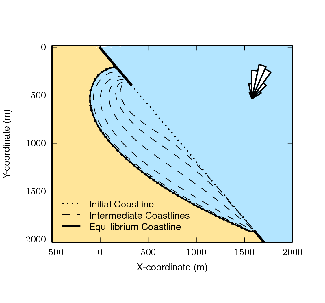
The model should then run for fifty years. This example evolves a crenulate-shaped bay from a straight initial coastline between two fixed headlands or sea walls. Sediment is transported out of the model domain by alongshore sediment flux and the shoreline gradually adjusts to the distribution of wave directions. The bay eventually reaches a state of equilibrium where the net alongshore flux is close to zero everywhere. The model is setup to run for 100 years, more than enough time for an equilibrium bay configuration to form.
While running the model will print the current model time to screen, it may also print some other messages, particularly including intersections in the coastline. The intersection analysis detects when the coastline intersects itself, such as when it erodes back behind the headland. Once this has happened the coastline is prevented from eroding any further.
4.2. Windows
4.2.1. Compiling and running: Code::Blocks
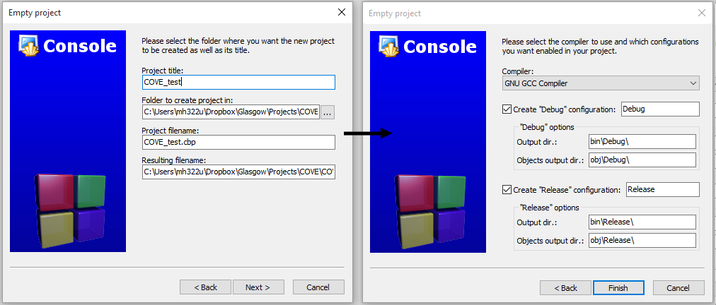
Since Code::Blocks is not the current development environment favoured by the COVE team, there is no Code::Blocks project file maintained in the COVE repository, and thus you will need to create one from scratch. Luckily, this process is pretty simple. Having opened Code::Blocks, from the startup click to create a new project:

Select the "Empty project" project template then click through the empty project creation wizard. You will be asked to name the project and provide a file/folder structure (see example) and then to select a compiler (select the GNU GCC Compiler; see example). Keep the default options for "Debug" and "Release" configurations and then click Finish.
|
Warning
|
You might have got an error message about the project not being able to save at this point, you can ignore it, the project appears to be saved. If you’re not sure about this, right click on the project within the Management side panel, and click Save project.
|
Next we need to populate the project with the required C++ files. From the top menu, click on Project → Add files… then navigate to the COVE repository directory. Add the following list of files to your project:
coastline.cpp, coastline.hpp
cliffline.cpp, cliffline.hpp
waveclimate.cpp, waveclimate.hpp
global_variables.hpp
./driver_files/spiral_bay_driver.cpp (1)
-
Or whichever driver file you wish to work with.
You should be able to expand the project in the Management side-bar to see these files organised by their file type (header or source).
To compile the code, from the top menu, click Build → Build. This will compile and link all of the code automatically and create an executable named YOUR_PROJECT_NAME.exe in the bin and debug folders of your project folder. You can then run the code from Code::Blocks by going to the top menu and clicking Build → Run. If the driver file you have chosen or created requires input arguments, these can be set by clicking Project → Set programs' arguments….
4.3. Plotting the results
We make plots of the resulting coastline evolution using the python matplotlib library. To use them you will need a python IDE such as Spyder. A series of plotting functions are included in the subdirectory plotting_functions. To plot the results of your spiral bay model run, open the file plot_coastline_evolution_figure.py in your favourite python IDE, and run. You should get the following figure:
Additionally, below will be a link to a video of a spiral bay evolving, which will be hosted on Vimeo once I have time to work out how to do it (MDH).
5. Example model runs
In this chapter we will look in detail at how the model is setup to perform a number of different example experiments. First we will look at the evolution of spiral bays from an initially straight coast line bound by sea walls or headlands, as used in Hurst et al. (2015). Next we will look at an example of an initially straight coastline using a periodic boundary condition subject to a mixture of low and high angle incidence offshore waves that generate hgih-angle wave instability, similar to the experiments of Ashton and Murray, 2006. Finally we will look at an example setup for a real stretch of cliffed coastline, using a stretch of the Suffolk coastline between Lowestoft and Southwold, which includes the interesting coastal foreland Benacre Ness. Hopefully this will give you some hands on guided experience of how to set the model up and how it behaves under different wave and boundary conditions.
5.1. Driver files
Each example model run has a driver file. Driver files are the files we will edit in order to control and customise COVE. The driver file initialises the coast, cliffs and waves and runs the coastal simulation following the control parameters that it contains.
5.1.1. Structure of a driver file
Declare Headers |
Manage Input Arguments (if any) |
Declare variables to control model run |
Initialise the coast, cliff and waves using variables |
Set model optional model parameters |
Setup output files |
Run Main Model Loop |
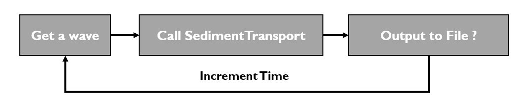
5.1.2. Structure of the main model loop
The model loop is pretty simple really, first grab a new wave from the wave climate, second pass it to the Coastline object when calling the TransportSediment function, third print the coordinates of the new Coastline to file.
And in code that looks something like this:
// loop through time and evolve the coast
while (Time < EndTime)
{
  //Get a new wave?
  if (Time > GetWaveTime)
  {
    MyWave = WaveClimate.Get_Wave();
    GetWaveTime += WaveTimeDelta/365.;
  }

  //Evolve coast
  CoastVector.TransportSediment(TimeStep, MyWave, CliffVector);

  //update time
  Time += TimeStep/365.;

  //Write results to file
  if (Time >= PrintTime)
  {
    CoastVector.WriteCoast(WriteCoastFile, Time);
    PrintTime += PrintTimeDelta;
  }
}
5.2. Spiral bays
Let’s look at how the model is set up to simulate the formation and evolution of crenulate-shaped bays (also known as spiral, log-spiral, zeta bays). To do so, we will open up the appropriate driver file and work through it to understand how the simulations are set up and what the model is doing.
5.2.1. The driver file
The driver file spiral_bay_driver.cpp can be found in the driver_files subdirectory. You can navigate to it and open in a text editor from the command line with:
$ cd driver_files
$ gedit spiral_bay_driver.cpp &
or open it from the explorer window.
OK, let’s look at the driver file. There are some helpful comments that are ignored when we run the program, these start with "//" or are in blocks "/*" to "*/". At the top of the file there are some #include statements that allow the program access to some libraries we will be using, including the model`s main coastline and waveclimate objects.
5.2.2. Setting up the wave climate
The spiral_bay_driver uses a Guassian representation of the wave climate. The parameters to set up the wave climate are required as input arguments at runtime. The wave climate is defined by a mean and standard deviation value for:
-
Wave period \(T\)
-
Wave height \(H_0\)
-
Wave direction \(\theta_0\)
and hence 6 input arguments are required. The driver file runs a check at the start to make sure it has the correct number of arguments, and will terminate with an error message if not.
In order to initialise the wave climate the 6 input arguments first are assigned to 6 variables:
//Declare parameter for wave conditions
double OffshoreMeanWavePeriod, OffshoreStDWavePeriod, OffshoreMeanWaveDirection, OffshoreStDWaveDirection, OffshoreMeanWaveHeight, OffshoreStDWaveHeight;
and the corresponding input arguments are converted from character sequences to numerical values and passed to these variables.
The wave climate is initialised by declaring a GuassianWaveClimate object called WaveClimate and passing these variables as input arguments in the correct order.
// initialise the wave climate
GaussianWaveClimate WaveClimate = GaussianWaveClimate(OffshoreMeanWavePeriod, OffshoreStDWavePeriod, OffshoreMeanWaveDirection, OffshoreStDWaveDirection, OffshoreMeanWaveHeight, OffshoreStDWaveHeight);
We then also declare an individual wave object. This holds the period, height and direction of an individual wave MyWave which we later pass to the coastline object in order to drive coastal evolution. We will sample a wave from WaveClimate and pass it to MyWave
// declare an individual wave (this will be sampled from the wave climate object
Wave MyWave = Wave();
// Get a wave from thewave climate object
MyWave = WaveClimate.Get_Wave();
5.2.3. Model run control parameters
Various parameters are required to control the length of the model run (in years), how often the coastline position is output to file (in years), how often to sample a new wave from the wave climate object (days), and how big the model timestep should be (days). We suggest leaving these as they are for now, but as you start customising model setup you may need to adjust them.
//declare time control paramters
int EndTime = 50.; // End time (years)
double Time = 0.; // Start Time (years)
double PrintTimeDelta = 36.5/365.; // how often to print coastline (years)
double PrintTime = PrintTimeDelta; // Print time (years)

double WaveTimeDelta = 0.1; // Frequency at which to sample new waves (days)
double GetWaveTime = 0.0; // Time to get a new wave (days)
double TimeStep = 0.05; // Time step (days)
5.2.4. Initialise the model
The spiral bay model is initialised as a straight coast with fixed boundaries at each end of the coast line. In order to generate the coastline object, we need to prescribe some attributes that dictate the properties of the generated coast, which we will pass to the new Coastline object when we declare it.
//initialise coast as straight line with low amp noise
int MeanNodeSpacing = 50; // in metres
double CoastLength = 2000; // in metres
double Trend = 140.; // in degrees

//boundary conditions are fixed
int StartBoundary = 2;
int EndBoundary = 2;-
MeanNodeSpacingsets approximately how widely spaced the Coastline cells will be. It is a mean value, because as the model evolves, nodes might get closer together or further apart, and nodes will be dynamically added or destroyed accordingly in order to maintain this average. -
CoastLengthis the length of the coastline between the fixed (or otherwise) end nodes. -
Trendis the orientation (azimuth) that the straight coastline should extend in.
|
Note
|
The sea is always on the left side of the vector, so imagine you are standing at node '[0]' looking down the vector. If the Trend is 140o then the sea is to the nort-east and the land to the south-west.
|
OK now that we have these variables in place we can go ahead and declare the Coastline object.
//initialise the coastline as a straight line
Coastline CoastVector = Coastline(MeanNodeSpacing, CoastLength, Trend, StartBoundary,
        EndBoundary);

//Initialise an empty/dummy cliffline object here
Cliffline CliffVector;
We declare a Coastline object whech we have called CoastVector, this is our coast, and all of its morphological properties are stored internally within the object. We provide the input arguments to the call in the order listed.
Note there is also a call to declare a Cliffline object called CliffVector. It has no input arguments and therefore generates an empty Cliffline object (i.e. there is no actual cliff line inside it). Our spiral bay experiments don`t require a cliffline object so that is OK, but this declaration is required to keep the model happy (it needs to be able to look at a cliff to know it doesn`t really exist, it`s a dummy cliff). Don`t worry about this for now, this will generate a warning when we come to run the model but we are OK to ignore it.
Finally, for our spiral bay runs, we want to allow some simple rules for the refreaction and diffraction of waves behind coastal obstructions to be operating. To do this we need to set a flag within the Coastline object, 1 = on, 0 = off.
// Allow refraction/diffraction rules
int RefDiffFlag = 1;
CoastVector.SetRefDiffFlag(RefDiffFlag);
Finally, before we run the main model loop, we’ll write the initial conditions to file:
// loop through time and evolve the coast
CoastVector.WriteCoast(WriteCoastFile, Time);
5.2.5. Main model loop
We’re all set up and ready to go! The model loop is pretty simple really, first grab a new wave from the wave climate, second pass it to the Coastline object when calling the TransportSediment function, third print the coordinates of the Coastline to file.
The model evolves until the Time exceeds the prescribed EndTime:
while (Time < EndTime)
{
        ...
We grab a new wave from the wave climate if it’s time (GetWaveTime depends on WaveTimeDelta which sets how often we get a new wave):
//Get a new wave?
if (Time > GetWaveTime)
{
        MyWave = WaveClimate.Get_Wave();
        GetWaveTime += WaveTimeDelta/365.;
}
Notice that GetWaveTime is in years, but WaveTimeDelta is in days, so we divide through by 365 to convert.
Now we evolve the coast by calling the Coastline function TransportSediment. This requires three input arguments, TimeStep is the length of time that sediment is transported over, we also give it the wave MyWave, and finally the dummy Cliffline object CliffVector:
//Evolve coast
CoastVector.TransportSediment(TimeStep, MyWave, CliffVector);
A whole lot of things happen inside this function (see a later section of this documentation that is yet to be written). The shoreline geometry is recalculated at each timestep. The wave is transformed from offshore to wave breaking conditions following linear wave theory, and any wave shadowing and refraction/diffraction are calculated. Alongshore sediment transport for each cell is calculated and the change in the volume of sediment in each cell calculated from the divergence of alongshore flux. The volume change is inverted for a change in the position of the coast and the position of each node is updated accordingly. The coastal geometry is updated for the next timestep.
There is a crude attempt written in here to allow adaptive timestepping. This hasn’t fully been tested yet, and usually if it’s called it’s because there is a bug in the model not actually associated with the adaptive timestep. If you run into this problem please email me.
Finally, the model prints the updated X and Y coordinates to an output file. See Writing Results to File for details of the resulting file format.
5.2.6. Compile and Run
Compile COVE for running a spiral bay by launching the makefile:
COVE/driver_files$ make -f spiral_bay_make.make
The file spiral_bay.out generated by compiling the code can be launched from the command line. The program takes the wave climate parameters as inputs \(T_{mean}\), \(T_{std}\), \(H_{mean}\), \(H_{std}\), \(\theta_{mean}\), \(\theta_{std}\):
COVE/driver_files$ ./spiral_bay.out 6 1 1. 0.1 35 25
The model should then run for fifty years. This example evolves a crenulate-shaped bay from a straight initial coastline between two fixed headlands or sea walls. Sediment is transported out of the model domain by alongshore sediment flux and the shoreline gradually adjusts to the distribution of wave directions. The bay eventually reaches a state of equilibrium where the net alongshore flux is close to zero everywhere. The model is setup to run for fifty years, more than enough time for an equilibrium bay configuration to form.
While running the model will print the current model time to screen, it may also print some other messages, particularly including intersections in the coastline. The intersection analysis detects when the coastline intersects itself, such as when it erodes back behind the headland. Once this has happened the coastline is prevented from eroding any further.
5.2.7. Plotting the results
A series of plotting functions are included in the subdirectory plotting_functions. To plot the results of your spiral bay model run, open the file plot_coastline_evolution_figure.py in your favourite python IDE, and run. You should get the following figure:
5.3. Cusps, Capes and Spits
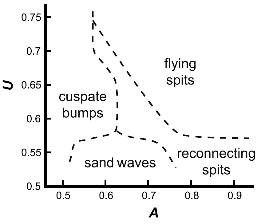
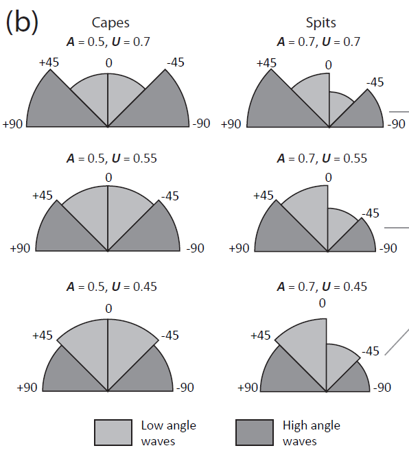
In this example, we will setup a model that simulates the formation of cusps, capes and spits, similar to the experiments of Ashton and Murray (2006). The type of coastal landform that the model produces depends on the nature of the wave climate used. Ashton and Murray (2006) developed a 4-bin approach to characterising offshore wave climates using two paramters; the proportion of waves that approach from high angle (U) and the proportion of waves that approach from the "left" (A), that is to say, the proportion of waves that would drive alongshore sediment transport down coast on a straight coastline (see section X for more info on this wave climate).
5.3.1. The driver file
The appropriate driver file is straight_periodic_driver.cpp and can be found in the driver_files subdirectory. You can navigate to it and open in a text editor from the command line with:
$ cd driver_files
$ gedit straight_periodic_driver.cpp &
or open it from the explorer window.
The driver file has been commented up helpfully to explain what is going on throughout. The driver file structure follows that laid out in section 5.1 (add link). We will assume you are already familiar with the spiral_bay_driver.cpp example.
5.3.2. Setting up the wave climate
Out straight, periodic boundary model run uses a UA wave climate, and hence 2 input arguments are required:
-
Wave direction highness (U)
-
Wave direction asymmetry (A)
Other wave parameters (period and height) are assigned explicitly within the driver file. The wave climate variables are assigned:
//Initialise real wave climate and temporary wave to pass
double U = atof(argv[1]);
double A = atof(argv[2]);
double OffshoreMeanWavePeriod = 6.;
double OffshoreStDWavePeriod = 1.;
double OffshoreMeanWaveHeight = 1.;
double OffshoreStDWaveHeight = 1.;
and these provide the corresponding input arguments for initialising the UAWaveClimate object. The wave climate is initialised by declaring a UAWaveClimate object called WaveClimate and passing it these variables as input arguments:
//initialise wave climate
UAWaveClimate WaveClimate = UAWaveClimate(U, A, Trend, OffshoreMeanWavePeriod, OffshoreStDWavePeriod, OffshoreMeanWaveHeight, OffshoreStDWaveHeight);
We then also declare an individual wave object. This holds the period, height and direction of an individual wave MyWave which we later pass to the coastline object in order to drive coastal evolution. We will sample a wave from WaveClimate and pass it to MyWave:
// declare an individual wave (this will be sampled from the wave climate object
Wave MyWave = Wave();
// Get a wave from thewave climate object
MyWave = WaveClimate.Get_Wave();
5.3.3. Model run control parameters
Similar to the spiral bay example, we need to declare parameters to control the length of the model run, how often we save results to file and when to sample new waves from the wave climate.
// DECLARATIONS
// These are the parameters that control the model run
//declare time control paramters
int EndTime = 100.; // End time (years)
double Time = 0.; // Start Time (years)
double PrintTimeDelta = 36.5/365.; // how often to print coastline (years)
double PrintTime = PrintTimeDelta; // Print time (years)

double WaveTimeDelta = 0.2; // Frequency at which to sample new waves (days)
double GetWaveTime = 0.; // Time to get a new wave (days)
double TimeStep = 0.2; // Time step (days)
double MaxTimeStep = 0.2; // Maximum timestep (days)
5.3.4. Initialise the model
There are two possible boundary types in COVE, fixed or periodic (at the moment). We want boundary conditions that are periodic, so sediment passed out of one end of the model is provided to the other. This means the end two nodes are geometric copies of each other and always experience the same amount of flux and change. We use an integer flag to specify boundary conditions, where 1 = periodic and 2 = fixed:
int StartBoundary = 1;
int EndBoundary = 1;
For periodic boundary condition runs initialise coast as straight line with a node spacing of 100 m and orientate the coast nort-south.
double Trend = 180.; // aximuth in degrees
int NodeSpacing = 100; // in metres
double CoastLength = 20000; // in metres
So now we can initialise the coastline as a straight line. With this call, we are creating a Coastline object which we will call CoastVector. To do this we need to provide this initialisation member function with 5 arguments so it can setup the coastline as we want it. We also create a Cliffline object, but because we do not assign it (there is no = sign), it will be completely empty (i.e. there is no cliff). When COVE checks to see whether there is a cliff to work with, it needs to see an empty cliff object to know that no cliff exists. I’d like to find a way to put thi "under the hood" but this will have to do for now.
//initialise the coastline as a straight line
Coastline CoastVector = Coastline(NodeSpacing, CoastLength, Trend, StartBoundary, EndBoundary);

// Initialise an empty/dummy cliffline object here.
Cliffline CliffVector;
The periodic coast expreiments do not require a Cliffline object but the declaration is required to keep the model happy. This will generate a warning when we initialise the model but we are OK to ignore it.
5.3.5. Set other model parameters
Next we need to set some other model parameters required to describe the shoreface and the style of sediment transport. There are a series of public set_ member functions that allow us to do this. Each of these have default values, so if you don’t set them the model will jsut use the defaults. The values we’re going to set here are the default values, just for illustrative purposes. They are
-
The Sediment flux flag (integer for which flux equation to use)
-
The refraction/diffraction flag (as set in the spiral bay example)
-
The shoreface depth (\(D_{sf}\); see Figure X)
-
The shoreface slope (\(\beta\); see Figure X)
First we will declare some temporary variables for these, and then call the functions to set them within the model:
// Declare variables
int CERCFlag = 1;
int RefDiffFlag = 0;
double ShorefaceDepth = 10.;
double ShorefaceSlope = 0.02;

// Call the set public member functions to control these parameters
CoastVector.SetRefDiffFlag(RefDiffFlag);
CoastVector.SetFluxType(CERCFlag);
CoastVector.SetShorefaceDepth(ShorefaceDepth);
CoastVector.SetShorefaceSlope(ShorefaceSlope);
5.3.6. Set up output file
We will automatically create an output file name based on the wave parameters provided as input arguments, and write the initial conditions to file uing the WriteCoast member function (see Writing Results to File section for more details).
//setup output file for writing results based on wave climate params
string arg1 = argv[1];
string arg2 = argv[2];
string underscore = "_";
string WriteCoastFile = "COVE" + underscore + arg1 + underscore + arg2 + ".xy";

// Write initial coast to file
CoastVector.WriteCoast(WriteCoastFile, Time);
5.3.7. Main model loop
This follows the same structure as outlined in section X.
5.3.8. Compile and Run
Compile COVE for running the straight, periodic coast example by launching the makefile:
COVE/driver_files$ make -f straight_periodic_make.make
This should create an executable file called Straight_Periodic.out which can be launched from the command line. The program requires two input arguments, U and A:
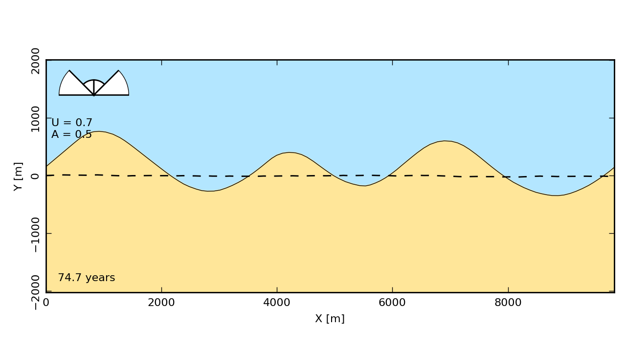
COVE/driver_files$ ./Straight_Periodic.out 0.7 0.5
This will run the model with 70% of waves coming from high angle, and 50% of waves coming from the north-east quadrant. This should result in the formation of sand waves that migrate down the coast (untested!). We should also be able to observe waves that migrate off the bottom of the model domain reappearing at the top.
While running the model will print the current model time to screen, and may also print some other messages recording unusual model behaviour!
5.3.9. Plotting the results
To plot the results of this run, we are going to create an animation! Open the file plot_periodic_animation.py in your favourite python IDE, and run. You should get a series of figures whose file names are numbered sequentially and each looks a bit like this:
The python script creates a file called filelist.txt which contains a list of all the output filenames. These frames can then be stitched together to create a video of the coastline evolving using Mencoder, a command line tool that is part of MPlayer that allows you to encode video files (Linux only). Thus once you have run the python script, you can run the following command to stich the output together into a nice video:
$ mencoder mf://@filelist.txt -mf w=300:h=600:fps=25:type=png -ovc lavc -lavcopts vcodec=mpeg4:mbd=2:trell -oac copy -o video.avi
Once you’ve made the video, you can delete all the individual png frame files to keep things tidy:
$ rm *.png
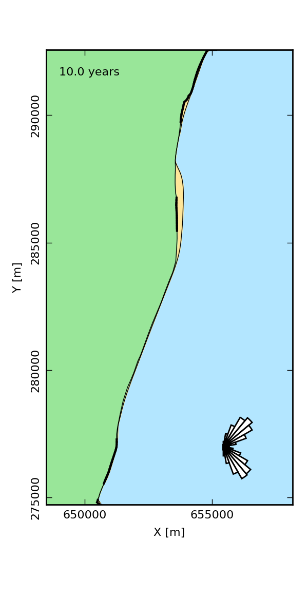
5.4. Real cliffed coast
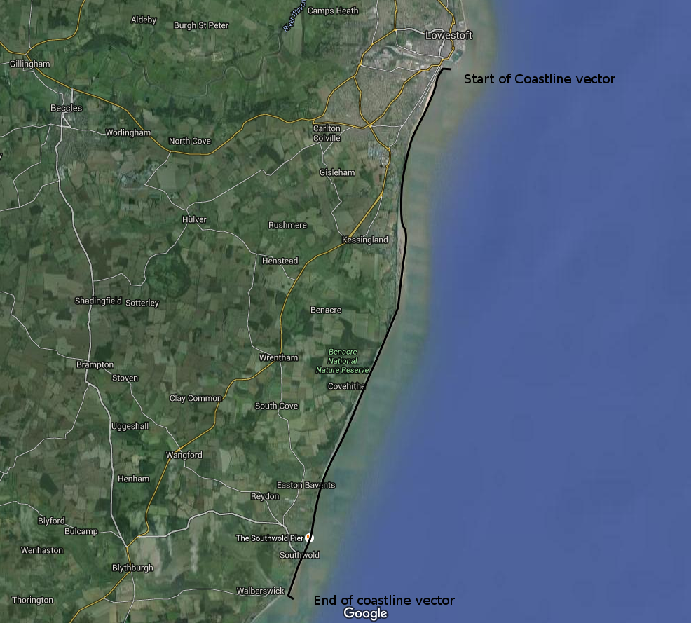
Let’s look at how to set the model up to run on a real stretch of cliffed coastline. The example we are going to look at is from the coast of Suffolk between Lowestoft and Southwold (see Figure 5).
Insert figure here of study site.
This coastline experiences a bimodal wave climate, with waves coming out of the North Sea to the north east, and through the English Channel from the South.
We are interested in this stretch of coastline because at Kessingland there is a large coastal foreland called Benacre Ness that is migrating northward along the coast. It is called Benacre Ness because it used to sit in front of the Benacre estate, but has migrated northward and now stretches across the frontage of Kessingland. It has been estimated to extend northward at rates of 20-50 m y-1, despite the locally established view that alongshore sediment transport is directed from north to south.
5.4.1. The driver file
The driver file benacre_driver.cpp can be found in the driver_files subdirectory. Hopefully the comments in the code will be helpful as you look through. These are ignored when the program is run. At the top of the file there are some #include statements that allow the program access to some libraries we will be using, including the model`s main coastline, cliffline and waveclimate objects.
5.4.2. Model run control parameters
Various parameters are required to control the length of the model run (in years), how often the coastline and cliffline positions are output to file (in years), how often to sample a new wave from the wave climate object (days), and how big the model timestep should be (days). We suggest leaving these as they are for now, but as you start customising model setup you may need to adjust them.
        //declare time control paramters
        int EndTime = 50.;        // End time (years)
        double Time = 0.;        // Start Time (years)
        double PrintTimeDelta = 36.5/365.;        // how often to print coastline (years)
        double PrintTime = PrintTimeDelta;        // Print time (years)

        double WaveTimeDelta = 0.2;        // Frequency at which to sample new waves (days)
        double GetWaveTime = 0.;        // Time to get a new wave (days)
        double TimeStep = 0.2;        // Time step (days)
        double MaxTimeStep = 0.2;        // Maximum timestep (days)
5.4.3. Input files
Using a real coastline, the model will require three input files in order to initialise the coast. A coastline x-y file, a cliffline x-y file and cliff type file. These are available in the example_inputs subdirectory of the repository. From the driver_file directory copy these across at the command line ready for running the model:
/COVE/driver_files/$ cp ../example_inputs/* .
These files have been declared in the driver file:
// initialise the coastline and cliffline objects from file
// first declare the filenames
string CliffInFile = "Benacre_Cliffline_Points.xy";
string CoastInFile = "Benacre_Coastline_Points.xy";
string FixedFileName = "Benacre_Fixed_Cliffs.data";
The coastline and cliffline *.xy files have the same format as the model output, consisting of a header line with two space-separated integers representing the start and end boundary conditions, followed by lines containing the x and y coordinates of the coastline, preceded by the time (see "Read a coast from file" in the "under the hood" section).
StartBoundary | EndBoundary
Time | X[0] | X[1] | X[2] =====> X[NoNodes]
Time | Y[0] | Y[1] | Y[2] =====> Y[NoNodes]
The order that your x and y coordinates come in is very important. The model ALWAYS assumes that the sea is on the left side as it works its way down the coastline or cliffline vector. To be sure you get this correct, imagine you are standing at the first node on your coastline, looking towards the second node. The sea will be on the left of the line, and the land on the right (see Figure 5). If this is backwards, you will get some very strange behaviour, because the model will ignore alot of waves (since they are coming from the land) and beach widths will be negative. If your first attempt at modelling a stretch of coastline blows up straight away, this is the first thing to check. We should probably write some error checking into the beach width calculator to flag negative values and warn you. This will get added in later.
The third file required is a cliff type file. This tells the model whether a cliff node can erode or is fixed (this can later be expanded to include different types of geology). Currently a value of 1 represents a fixed coast (e.g. defended by sea wall/revetment) and a value of 0 is a normal erodible cliff. The file format is a header line followed by two columns, one for the node index (i=0 to i=NoNodes-1) and the second for the cliff type integer.
Index Type
0 1
1 0
2 0
...
NoNode-1 1
5.4.4. Wave climate
Wave data from the Southwold wave buoy shows that our example coast is hit by a bimodal wave climate. The wave buoy is in 25 m water depth and suggests high angle waves impinging toward the coast, which if fed directly to the model results in high angle wave instability that is not observed on this stretch of coastline. A legacy data set from a previously deployed AWAC wave buoy shows that these dominant wave modes get rotated to lower angle of incidence by the time they reach the shoreface, so for these example experiments, we have chosen a similar lower angle, bimodal wave climate.
Our bimodal wave climate consists of two Gaussian wave climates as used in the spiral bay experiments. The parameters for these have been declared in the driver file diectly rather than being passed as input arguments.
// Bimodal wave climate
//Wave climate 1
double OffshoreMeanWaveDirection1 = 45.;
double OffshoreStDWaveDirection1 = 20.;
double OffshoreMeanWavePeriod1 = 6.;
double OffshoreStDWavePeriod1 = 2.;
double OffshoreMeanWaveHeight1 = 0.8;
double OffshoreStDWaveHeight1 = 0.2;
GaussianWaveClimate WaveClimate1(OffshoreMeanWavePeriod1,OffshoreStDWavePeriod1,OffshoreMeanWaveDirection1,OffshoreStDWaveDirection1,OffshoreMeanWaveHeight1, OffshoreStDWaveHeight1);

//Wave climate 2
double OffshoreMeanWaveDirection2 = 140.;
double OffshoreStDWaveDirection2 = 20.;
double OffshoreMeanWavePeriod2 = 5.;
double OffshoreStDWavePeriod2 = 1.;
double OffshoreMeanWaveHeight2 = 1.1;
double OffshoreStDWaveHeight2 = 0.2;
GaussianWaveClimate WaveClimate2(OffshoreMeanWavePeriod2,OffshoreStDWavePeriod2,OffshoreMeanWaveDirection2,OffshoreStDWaveDirection2,OffshoreMeanWaveHeight2, OffshoreStDWaveHeight2);
So we have two wave climate objects, WaveClimate1 and WaveClimate2. As before we also need to declare an individual wave object:
//declare wave
Wave MyWave = Wave();
MyWave = WaveClimate1.Get_Wave();
In the main model loop, we will use a random number generate to select which wave climate to grab a wave from at random, and assign it to MyWave ready to evolve the coast.
5.4.5. Initialisation
We initialise both the coastline and the cliffline objects by pointing them to the respective input files as detailed in the previous subsection. We then provide an extra call to the CliffVector object to tell it to read whether the cliff is fixed or erodible:
// Read the coastline and cliffline data from files
double StartTime = 0;
Cliffline CliffVector = Cliffline(CliffInFile, StartTime);
Coastline CoastVector = Coastline(CoastInFile, StartTime);

// Load data on cliff type (fixed vs erodible)
CliffVector.ReadCliffType(FixedFileName);
Then we declare a couple more file names where we will write the output files for both the cliffline and the coastline object:
//declare output file names
string WriteCoastFile = "CliffedCoast_Coastline.xy";
string WriteCliffFile = "CliffedCoast_Cliffline.xy";
There are a few other things we need to set up for this run; how fast the cliffs can erode, how high the cliffs are, what the critical beach width is that maximises cliff erosion, and how much cliff material gets lost offshore when the cliff erodes.
First, we will setup the maximum retreat rate. This is the fastest retreat rate the cliffs can manage, and can be informed or calibrated by historical observations of cliff retreat. For our section of the Suffolk coast, we will set this to 5 m yr-1, guided by Brooks and Spencer (2010).
// Set Maximum Retreat Rate (m/yr)
// This is E0 for the Valvo et al. (2006) or Limber and Murray (2011) models of cliff erosion
double RetreatRate = 5.;
CliffVector.SetMaxRetreatRate(RetreatRate);
Second, we will set the cliff height. At the moment this is spatially and temporally continuous, but functionality can be added later to extract this value from a DEM as the model evolves.
// Set Cliff Height (m)
// Fixed for now, but could in the future grab this from a DEM
double CliffHeight = 10.;
CliffVector.SetCliffHeight(CliffHeight);
Third, we set the critical beach width. This is the beach width at which the maximum rate of cliff retreat occurs. For wider beaches, the rate of cliff retreat declines exponentially. We will set this to 5 m, suggesting that a 5 m wide beac provides the optimal balance between protecting the cliff and providing abrasive tools such that cliff erosion is maximised.
// Set critical beach width (m)
// The beach width that maximises the rate of cliff retreat E0
double CriticalBeachWidth = 5.;
CliffVector.SetCriticalWidth(CriticalBeachWidth);
Fourth, we set the style of cliff retreat. ErosionType = 1 if using a Valvo et al. (2006) type of relationship between beach width and cliff retreat (this is effectively the same as setting CriticalBeachWidth = 0 and thus redundant). 'ErosionType = 2' uses the Limber and Murray (2011) relationship between beach width and cliff retreat where cliff retreat rate peaks at CriticalBeachWidth.
// For Valvo Style Cliff Retreat ErosionType = 1,
// for Limber and Murray ErosionType = 2
int ErosionType = 1;
Fifth, we set the proportion of cliff material assumed to be lost to the sea:
// Set lost cliff fraction
// The proportion of cliff material that is lost offshore by suspension
double LostFraction = 0.2;
CliffVector.SetLostFraction(LostFraction);
And finally, since the Suffolk beaches are mixed sand/shingle, we tell the coastline object to use an alongshore flux equation that has been modified to better reflect gravel transport rates:
// Set lost cliff fraction
// The proportion of cliff material that is lost offshore by suspension
double LostFraction = 0.2;
CliffVector.SetLostFraction(LostFraction);
5.4.6. Main model loop
Good to go! The model loop is pretty simple really, first grab a new wave at random from one of the two wave climates, second pass it to the Coastline object when calling the TransportSediment function, third call the Cliffline object’s ErodeCliff function, and finally print the coordinates of both the Coastline and Cliffline to file.
The model evolves until the Time exceeds the prescribed EndTime:
while (Time < EndTime)
{
        ...
We grab a new wave from the wave climate if it’s time (GetWaveTime depends on WaveTimeDelta which sets how often we get a new wave):
//Get a new wave?
if (Time > GetWaveTime)
{
        // Use a random sampler to chose between wave climates
        rand1 = (double)rand()/RAND_MAX;
        if (rand1 < 0.5) MyWave = WaveClimate1.Get_Wave();
        else MyWave = WaveClimate2.Get_Wave();
        GetWaveTime += WaveTimeDelta/365.;
}
rand1 selects a random number between 0 and 1. When rand1 < 0.5 we use WaveClimate1 and otherwise we use WaveClimate2 so we should be sampling equally from both wave climates. Notice that GetWaveTime is in years, but WaveTimeDelta is in days, so we divide through by 365 to convert.
Now we evolve the coast by calling the Coastline function TransportSediment, followed by the Cliffline function ErodeCliff. Each requires three input arguments. For the Coastline.TransportSediment call, TimeStep is the length of time that sediment is transported over, we also give it the wave MyWave, and finally the Cliffline object CliffVector so that it can only erode beach material that fronts the cliff. For the Cliffline.ErodeCliff call, we pass TimeStep again, the Coastline object, and the type of erosion law ErosionType.
//Evolve coast
CoastVector.TransportSediment(TimeStep, MyWave, CliffVector);
CliffVector.ErodeCliff(TimeStep, CoastVector, ErosionType);
A whole lot of things happen inside these functions (see a later section of this documentation that is yet to be written). Coastline and Cliffline geometry is recalculated at each timestep. The wave is transformed from offshore to wave breaking conditions following linear wave theory, and any wave shadowing and refraction/diffraction are calculated. Alongshore sediment transport for each cell is calculated and the change in the volume of sediment in each cell calculated from the divergence of alongshore flux, checking with the Cliffline position that sediment is available for transport. The volume change is inverted for a change in the position of the coast and the position of each node is updated accordingly. The coastal geometry is updated for the next timestep. The width of the beach is calculated by comparing the Coastline and Cliffline objects and this determines the amount of cliff retreat. The Cliffline position is updated and the amount of volume lost is supplied to the adjacent beach, minus the amount lost to the sea.
Finally, the model prints the updated X and Y coordinates to two output files. See Writing Results to File for details of the resulting file format.
5.4.7. Compile and run
Compile COVE for running the Suffolk example by launching the makefile:
COVE/driver_files$ make -f benacre_make.make
The file benacre.out generated by compiling the code can be launched from the command line without any input arguments :
COVE/driver_files$ ./benacre.out
The model should then run for fifty years. This example evolves the Suffolk coast such that the cuspate foreland Benacre Ness migrates northward up the coast at rates in keeping with historical observations. While running the model will print the current model time to screen.
5.4.8. Plotting the results
A series of plotting functions are included in the subdirectory plotting_functions. To plot the results of your Suffolk model run, open the file benacre_evolution_animation.py in your favourite python IDE, and run. You should get a series of figures whose file names are numbered sequentially and each looks a bit like this:
The python script creates a file called filelist.txt which contains a list of all the output filenames. These frames can then be stitched together to create a video of the coastline evolving using Mencoder, a command line tool that is part of MPlayer that allows you to encode video files. Thus once you have run the python script, you can run the following command to stich the output together into a nice video:
$ mencoder mf://@filelist.txt -mf w=300:h=600:fps=25:type=png -ovc lavc -lavcopts vcodec=mpeg4:mbd=2:trell -oac copy -o video.avi
Once you’ve made the video, you can delete all the individual png frame files to keep things tidy:
$ rm *.png
6. Wave Climates
The model requires wave conditions to drive alongshore sediment transport. This is supplied in the form of a waveclimate object that the coastline model can interact with. For the purposes of this model, a wave climate consists of a timeseries of waves considered to be "offshore", that is to say the wave conditions recieved at the bottom of the shoreface. This time series comprises significant wave height \(H_0\), wave period \(T\) and wave direction \(\theta_0\). The waveclimate object can take a variety of guises, including both hypothetical and real wave climates. the model is most sensitive to variation in wave direction. Hypothetical wave climates include the U-A descripition of wave directions (Ashton & Murray, 2006) or a simple Gaussian distribution (Hurst et al., 2015). Real wave climates read in a timeseries of \(H_0\), \(T\) and \(\theta_0\) data that might be collected from a nearby wave buoy deployment, or generated by a coastal area model such as FVCOM or SWAN.
6.1. Single wave
The Wave object describes a single wave, and contains the wave period \(T\), height \(H_0\) and direction \(\theta_0\). The single wave object can be used as the entire wave climate but is more commonly implemented as an object sampled from another distributed wave climate. An individual wave can be declared and used to sample a wave from an existing wave climate as seen here:
// declare an individual wave (this will be sampled from the wave climate object
Wave MyWave = Wave();
// Get a wave from the wave climate object
MyWave = WaveClimate.Get_Wave();
A new single wave object may be sampled during the main model loop at the desired time step:
while (Time < EndTime)
{
  //Get a new wave?
  if (Time > GetWaveTime)
  {
    MyWave = WaveClimate.Get_Wave();
    GetWaveTime += WaveTimeDelta/365.;
  }
  ...
6.2. Gaussian wave climate
The GuassianWaveClimate object contains six parameters to describe distributions of Wave period \(T\), Wave height \(H_0\), and Wave direction \(\theta_0\). In order to initialise the wave climate in a driver file, 6 variables must be declared, and values assigned:
//Declare parameter for wave conditions
double OffshoreMeanWavePeriod, OffshoreStDWavePeriod, OffshoreMeanWaveDirection,
        OffshoreStDWaveDirection, OffshoreMeanWaveHeight, OffshoreStDWaveHeight;
The wave climate is initialised by declaring a GuassianWaveClimate object called WaveClimate and passing these variables as input arguments in the correct order.
// initialise the wave climate
GaussianWaveClimate WaveClimate = GaussianWaveClimate(OffshoreMeanWavePeriod,
        OffshoreStDWavePeriod, OffshoreMeanWaveDirection, OffshoreStDWaveDirection,
        OffshoreMeanWaveHeight, OffshoreStDWaveHeight);
We then also declare an individual wave object. This holds the period, height and direction of an individual wave MyWave which we later pass to the coastline object in order to drive coastal evolution. We will sample a wave from WaveClimate and pass it to MyWave
// declare an individual wave (this will be sampled from the wave climate object
Wave MyWave = Wave();
// Get a wave from the wave climate object
MyWave = WaveClimate.Get_Wave();
This last line should appear in the main model loop to select new waves at the chosen frequency:
while (Time < EndTime)
{
  //Get a new wave?
  if (Time > GetWaveTime)
  {
    MyWave = WaveClimate.Get_Wave();
    GetWaveTime += WaveTimeDelta/365.;
  }
  ...
6.3. Bimodal wave climate
A bimodal wave climate can be created by using two other wave climate objects such as the Gaussian wave climate, and sampling between the two at random. To set up such a model, first declare two Gaussian wave climates with the chosen parameters:
// Bimodal wave climate
//Wave climate 1
double OffshoreMeanWaveDirection1 = 45.;
double OffshoreStDWaveDirection1 = 20.;
double OffshoreMeanWavePeriod1 = 6.;
double OffshoreStDWavePeriod1 = 2.;
double OffshoreMeanWaveHeight1 = 0.8;
double OffshoreStDWaveHeight1 = 0.2;
GaussianWaveClimate WaveClimate1(OffshoreMeanWavePeriod1,OffshoreStDWavePeriod1,OffshoreMeanWaveDirection1,OffshoreStDWaveDirection1,OffshoreMeanWaveHeight1, OffshoreStDWaveHeight1);

//Wave climate 2
double OffshoreMeanWaveDirection2 = 140.;
double OffshoreStDWaveDirection2 = 20.;
double OffshoreMeanWavePeriod2 = 5.;
double OffshoreStDWavePeriod2 = 1.;
double OffshoreMeanWaveHeight2 = 1.1;
double OffshoreStDWaveHeight2 = 0.2;
GaussianWaveClimate WaveClimate2(OffshoreMeanWavePeriod2,OffshoreStDWavePeriod2,OffshoreMeanWaveDirection2,OffshoreStDWaveDirection2,OffshoreMeanWaveHeight2, OffshoreStDWaveHeight2);
Then declare an individual wave object:
// declare an individual wave (this will be sampled from the wave climate object
Wave MyWave = Wave();
// Get a wave from the wave climate object
MyWave = WaveClimate.Get_Wave();
In the main model loop we will use a random number generator to choose which of the two wave climates to select from. The fraction 0.5 dictates that we should sample roughly half of the waves from each wave climate. This could be adjusted if it was required that one mode should be more dominant.
while (Time < EndTime)
{
        //Get a new wave?
        if (Time > GetWaveTime)
        {
                // Use a random sampler to chose between wave climates
                rand1 = (double)rand()/RAND_MAX;
                if (rand1 < 0.5) MyWave = WaveClimate1.Get_Wave();
                else MyWave = WaveClimate2.Get_Wave();
                GetWaveTime += WaveTimeDelta/365.;
        }
        ...
6.4. U-A wave climate
Ashton and Murray (2006) used a 4-bin directional wave climate to represent offshore waves that will interact with the coastline. This four-bin directional wave climate can be described by two parameters, wave direction highness U and asymmetry A: * the fraction of waves that approach from high angle U (>45o relative to the overall trend of the coastline) * the fraction of waves that approach from the "left" A (i.e. up coast)
Here are some example plots of 4-binned wave climates and their associated U and A values to illustrate (after Thomas et al. 2016):
To declare the wave climate, we also need values for the mean and standard deviation for wave period latexmath:[T] and wave height latexmath:[H_0]. Thus we declare:
double U = 0.55;
double A = 0.7;
double OffshoreMeanWavePeriod = 6.;
double OffshoreStDWavePeriod = 1.;
double OffshoreMeanWaveHeight = 1.;
double OffshoreStDWaveHeight = 1.;
A UAWaveClimate object with U = 0.55 and A = 0.7 can then be declared and assigned to an object called WaveClimate by passing these variables:
//initialise wave climate
UAWaveClimate WaveClimate = UAWaveClimate(U, A, Trend, OffshoreMeanWavePeriod, OffshoreStDWavePeriod, OffshoreMeanWaveHeight, OffshoreStDWaveHeight);
We then also declare an individual Wave object. This holds the period, height and direction of an individual wave MyWave which we later pass to the coastline object in order to drive coastal evolution. We will sample a wave from WaveClimate and pass it to MyWave:
// declare an individual wave (this will be sampled from the wave climate object
Wave MyWave = Wave();
// Get a wave from the wave climate object
MyWave = WaveClimate.Get_Wave();
The last line will appear inside the main model loop in the driver file to select new waves at each or the specified model time step:
while (Time < EndTime)
{
  //Get a new wave?
  if (Time > GetWaveTime)
  {
    MyWave = WaveClimate.Get_Wave();
    GetWaveTime += WaveTimeDelta/365.;
  }
  ...
6.5. Real wave data
The model can be driven by wave data such as that taken from a wave buoy or supplied from an external wave model such as FVCOM or SWAN. The required input parameters are offshore wave direction, period and height.
Input files should have a header line, and three data columns for direction, period and height.
Headers
   Dir[0]    |    Period[0]    |    Height[0]
   Dir[1]    |    Period[1]    |    Height[1]
   Dir[2]    |    Period[2]    |    Height[2]
    ...      |       ...       |      ...
Dir[NoWaves] | Period[NoWaves] | Height[NoWaves]
The model doesn’t read how frequent the data are, but the frequency with which the model samples this data can be set in a driver file. The data is read and sampled in the order provided.
The wave climate is initialised in a driver file by passing the input filename as a string:
// initialise the wave climate
WaveFileName = "MyWaveData.txt";
RealWaveClimate WaveClimate = RealWaveClimate(WaveFileName);
An individual wave object will also be required:
// declare an individual wave (this will be sampled from the wave climate object
Wave MyWave = Wave();
A wave is then sampled from the wave climate by assigning it the individual wave object:
// Get a wave from the wave climate object
MyWave = WaveClimate.Get_Wave();
Note that the model will proceed iteratively through the wave climate data until it reaches the end of the file, then will loop back to the beginning and keep going continously until the model run is ended.
7. Under the hood
This section still has a long way to go!
7.1. Initialising a Coastline object
7.1.1. Read a Coastline from file
Input files for the position of the coast take the same format as output files. The first line is a header containing integer values for the StartBoundary and EndBoundary conditions. The next two lines are the X and Y coordinates of the line respectively, but both preceded by the time (in years). We use \| to indicate a white space delimiter here such as a space or tab.
StartBoundary | EndBoundary
Time | X[0] | X[1] | X[2] =====> X[NoNodes]
Time | Y[0] | Y[1] | Y[2] =====> Y[NoNodes]
So for example, a 5 metre long coastline with fixed boundary conditions oriented at 135^o with a \(sqrt{2}\) node spacing, at Time = 0 would have an input file:
2 2
0 0 1 2 3 4 5
0 0 1 2 3 4 5
7.2. Initialising a Cliffline object
7.3. Boundary Conditions
The model is a single line. The start and end of the line can be handled in different ways. At the moment, we have two possible boundary conditions, which are assigned by setting the StartBoundary and EndBoundary parameters when initialising the coastline, or putting these in the header of an input file if initialising the coastline with an existing coastline output file (or real coastline). The boundary conditions are set by an integer as:
1. Periodic boundary conditions: the start of the line is also the end, and sediment can be passed \"round the back\" e.g. an island.
2. Fixed boundary conditions the first and last two nodes/cells in the model are fixed and immovable.
7.4. Writing results to file
The Coastline object writes the position of the coast to a text file with a name provided in the call WriteCoastFile. The Time must also be passed:
//loop through time and evolve the coast
CoastVector.WriteCoast(WriteCoastFile, Time);
The file format is the same as for reading a coast from a text file. The first line is a header containing integer values for the StartBoundary and EndBoundary conditions. The next two lines are the X and Y coordinates of the line respectively, but both preceded by the time (in years). We use \| to indicate a white space delimiter here such as a space or tab.
StartBoundary | EndBoundary
Time | X[0] | X[1] | X[2] =====> X[NoNodes]
Time | Y[0] | Y[1] | Y[2] =====> Y[NoNodes]
So for example, a 5 metre long coastline with fixed boundary conditions oriented at 135^o with a \(sqrt{2}\) node spacing, at Time = 1, that has not changed since Time = 0 would have an input file:
2 2
0 0 1 2 3 4 5
0 0 1 2 3 4 5
1 0 1 2 3 4 5
1 0 1 2 3 4 5
More details to follow. See the [Doxygen documentation] for the time being.
8. Ensemble mode
Details to follow.
Appendix A: Debugging
This model is a developing research tool and may contain bugs or behave in an unexpected manner as new applications and study sites are tested and as code development is continues. Statements have been written into the model code to print to screen when unusual behaviour occurs, telling you where in the code this has happened, what the problem is, and what (if anything) the model has done to try and resolve the problem.
Coastline: Initialising Coastline as straight segment
	 MeanNodeSpacing = 50
	 CoastLength = 2000
	 Boundary Conditions = 2, 2


Cliffline.Initialise: Warning, initialised an empty Cliffline object
Coastline: Time is 1.10 years
In TransportSediment at line 3829: Large Position Change, reducing timestep!
In TransportSediment at line 3829: Large Position Change, reducing timestep!
In TransportSediment at line 3829: Large Position Change, reducing timestep!
For example in the output above, we have recieved a warning that there is an empty Cliffline object (this is fine in certain circumstances), and a notification that a large position change in the coast has occurred. This is usually an indication that you need to reduce your model timestep, but may sometimes be indicative of some other problem within the model and is worthy of exploration.
Often the best way to diagnose such a problem further, or understand what might be happening when the model fails to run completely, is to run the model in debug mode. Debug mode allows you to stop the model at any point, query what is going on, query the values of variables or find out exactly where and why the model fell over.
A.1. The GNU Debugger (GDB)
During model development, debugging has principally taken place in the GNU debugger (GDB). GDB is a command line tool for executing and controlling a model run within a debugging environment. Useful functionality includes the ability to: .pause and continue the model at any point, including where certain conditions are met, .catch memory dumps, segmentation faults, stack overflows, memory leaks etc. in the act, .print where abouts within the model structure the model is currently executing, .print the value of any variables or memory location to screen.
Here, we will go through some basic commands to get started with debugging using GDB. More extensive instructions and examples can be found in abundance online, see for example GDB Cheat Sheet.
A.1.1. Running GDB
The makefiles used for compiling COVE typically include the required flags to allow GDB to function correctly (you have to tell your compiler that you want to debug when you compile the code). To launch GDB for compiling a particular model (e.g. the spiral bay model executable), run the command:
$ gdb spiral_bay.out
You will be presented with the (gdb) console from which you can make commands to the debugger.
A.1.2. Running the model in debug model
To run the model in debug mode, type run, followed by any required commandline arguments:
(gdb) run 6 1 1. 0.1 35 25
The model will execute as if you launched it from the command line, and all being well will complete. If you have already run the model once inside the current debug session, you can rerun by just typing run, without the additional arguments, and it will execute with the same arguments as the previous run.
A.1.3. Pausing and resuming the modeling
If you’d like to pause the model while it is running, press CTRL-C on your keyboard. You will be returned to the (gdb) console. To resume the model, type c at the console. When paused this way, we have no idea where abouts within the model it is paused.
A.1.4. Backtracing to find out where we are
We can find out where in the model we have got to by typing:
(gdb) backtrace
This will print to screen a history of where the model has been to get to where it is currently:
#0  Coastline::TransportSediment (this=0x7fffffffd900, TimeDelta=@0x7fffffffd520: 0.10000000000000001,
    TheWave=..., CliffVector=...) at ../coastline.cpp:3838
#1  0x000000000043d7c5 in main () at spiral_bay_driver.cpp:144
This is telling us the model is #1 inside the main function of spiral_bay_driver.cpp at line 144. This happens to be the TransportSediment function, and #0 tells us that it is at line 3838 within that function in the 'coastline.cpp' file.
The backtrace function can be particularly useful for pinpointing where memory leaks and segmentation faults have occurred if the model fails for one of these reasons.
A.1.5. Setting break points
Before executing the model, or whilst paused, we can set up break points to tell the model to stop when it reaches a certain place in the code. For example:
(gdb) break spiral_bay_driver.cpp:186
Breakpoint 1 at 0x424a16: file ../spiral_bay_driver.cpp, line 186.
This tells the debugger to automatically break (pause) the model whenever line 186 in the spiral_bay_driver.cpp file is reached. This has been assigned a number Breakpoint 1.
A.1.6. Conditional break points
You can tell the debugger to only implement the break point if a particular conditions is met, using the same conditional syntax as you would use in C++ code. In the next command, we’ll tell the model to break when the variable Time is greater than 0.1, using the cond command, telling it to apply to Breakpoint 1, and telling it what the conditional statement is:
(gdb) cond 1 Time > 0.1
(gdb) c
Typing c for continue, or run to run/rerun the model will execute the model until this condition is met, upon which the model will pause/break.
A.1.7. Printing variables to screen
In the case above, line 186 happens to be inside the main model loop. To see how much model time has elapsed, we can use the print (or p for short) command to display the Time variable on screen:
(gdb) p Time
$1 = 0.1001
Telling us that Time has a value of 0.1. We can also access and print values from within objects, such as the coastline object called CoastVector. Let’s print the number of nodes in our coastline object:
(gdb) p CoastVector.NoNodes
$2 = 57
So there are 57 nodes. Another way you can find out how many nodes there are would be using
(gdb) p X.size()
$3 = 57
The coastline object CoastVector contains a variety of vectors, such as the Orientation vector. To print the whole vector, simply type:
(gdb) p Orientation
$9 = std::vector of length 57, capacity 57 = {315, 321.60094533591007, 22.216282736864009,
  337.92083201072523, 331.46683943535487, 328.74000871549521, 328.56943628252139, 329.3837844925842,
  331.03563876766952, 332.40559792862649, 332.82638125188163, 332.9245341437483, 332.93052241718527,
  332.89505726491376, 332.83385098343905, 332.74888832616358, 332.64670360927767, 332.51956294297577,
  332.37435404622971, 332.19187033915836, 331.98128493122556, 331.73952655625015, 331.45574672016079,
  331.12294086709244, 330.75626492842684, 330.33227946333, 329.8343696059797, 329.28977634602285,
  328.55965087010219, 327.69635559935881, 326.64424950907846, 325.53196699095071, 324.23753352499017,
  322.87152718696478, 321.28662654854742, 319.48794541733355, 317.39883969083547, 315.31314397231881,
  312.5481246023183, 309.3840749386398, 305.72483950877961, 300.26574163061139, 294.0715726264682,
  287.02711087458448, 278.49458640312565, 270.15845682076986, 259.64212073586492, 250.94017797254546,
  239.4529514946729, 226.11779089145259, 210.20538031715429, 191.46362690977978, 169.54150518072848,
  146.8206916976348, 134.99530456698648, 315.00076908588517, 315.00076908588517}
If you jsut want to know what the Orientation of the first node or last node is, try:
(gdb) p Orientation[0]
$10 = 315
(gdb) p Orientation[NoNodes-1]
$11 = 315.00076908588517
9. References
Ashton, A. D., and A. B. Murray (2006), High-angle wave instability and emergent shoreline shapes: 1. Modeling of sand waves, flying spits, and capes, J. Geophys. Res., 111, F04011, doi: 10.1029/2005JF000422.
Barkwith, A., Thomas, C. W., Limber, P. W., Ellis, M. A., and Murray, A. B. (2014a), Coastal vulnerability of a pinned, soft-cliff coastline – Part I: Assessing the natural sensitivity to wave climate, Earth Surf. Dynam., 2, 295-308, doi: 10.5194/esurf-2-295-2014.
Barkwith, A., Hurst, M. D., Thomas, C. W., Ellis, M. A., Limber, P. L., and Murray, A. B. (2014b) Coastal vulnerability of a pinned, soft-cliff coastline, II: assessing the influence of sea walls on future morphology, Earth Surf. Dynam., 2, 233-242, doi: 10.5194/esurf-2-233-2014.
Brooks, S. M., and T. Spencer (2010), Temporal and spatial variations in recession rates and sediment release from soft rock cliffs, Suffolk coast, UK, Geomorph., 124, 26-41, doi: 10.1016/j.geomorph.2010.08.005.
Hurst, M. D., A. Barkwith, M. A. Ellis, C. W. Thomas, and A. B. Murray (2015), Exploring the sensitivities of crenulate bay shorelines to wave climates using a new vector-based one-line model, J. Geophys. Res. Earth Surf., 120, 2586–2608, doi: 10.1002/2015JF003704.
Limber, P. W. and A. Brad Murray (2011) Beach and sea-cliff dynamics as a driver of long-term rocky coastline evolution and stability, Geology, 39, 1147-1150, doi: 10.1130/G32315.1
Thomas, C. W., Murray, A. B., Ashton, A. D., Hurst, M. D., Barkwith, A. K. A. P., and Ellis, M. A. (2016), Complex coastlines responding to climate change: do shoreline shapes reflect present forcing or "remember" the distant past?, Earth Surf. Dynam. Discuss., doi: 10.5194/esurf-2016-35, in review.
Valvo, L. M., A. B. Murray, and A. Ashton (2006), How does underlying geology affect coastline change? An initial modeling investigation, J. Geophys. Res., 111, F02025, doi: 10.1029/2005JF000340